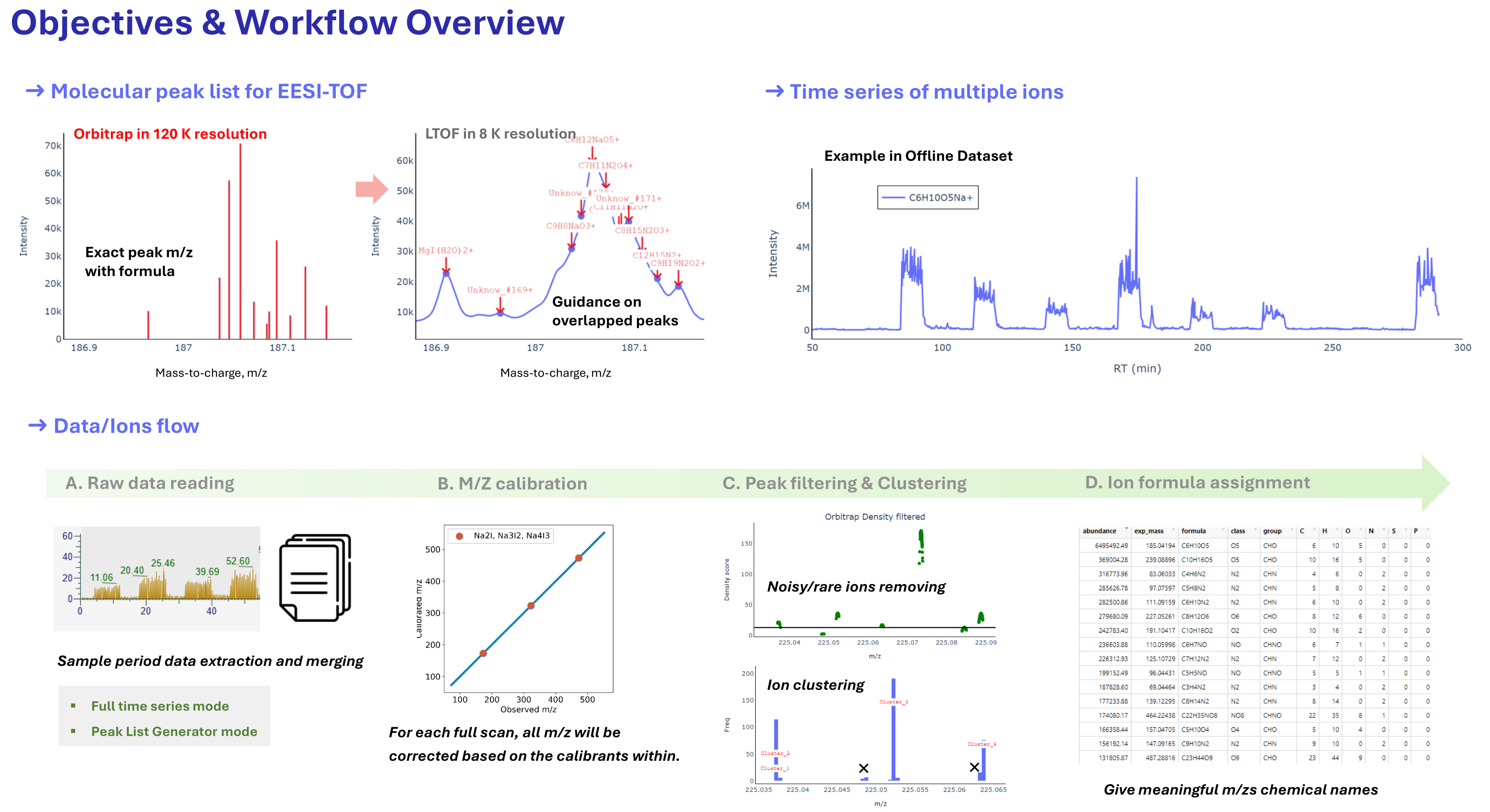
The ultra-high resolution of Orbitrap mass spectrometry enables an unprecedented level of chemical detail. In my current research, we employ a direct-infusion Orbitrap approach (EESI inlet, Felipe et al, 2019) for non-targeted analysis. However, due to the lack of dedicated tools tailored for this application, I developed a new software package called OrbiTrack. This tool supports two core workflows:
(1) TOF peak guidance: Guiding ion fitting in EESI-TOF using high-resolution chemical information acquired at 120k resolution from Orbitrap.
(2) Directly utilization of Orbitrap MS1 data by integrating full time-series MS1 outputs, enabling online untargted molecular analysis without chromatographic sepeartion.
This blog series will introduce the OrbiTrack framework step by step, covering the conceptual foundations and sharing the original scripts for each component:
TOF integration/refiner (optional, used when leveraging Orbitrap-resolved ions to support TOF fitting) link
Feedback and suggestions are highly welcome. Feel free to leave a comment below or contact me via email.
In this first post, I will introduce Part 1: loading Orbitrap raw MS1 data by user-defined time period.
1. Orbitrap Working Principle
Before diving into the code examples, I’ll first summarize the Orbitrap data format and its underlying principles. This not only helps me organize my own understanding but may also be useful for others new to Orbitrap data processing.
Orbitrap raw data can be conceptually understood as a sequence of dataframes, each corresponding to a snapshot in time. Each individual dataframe contains a list of m/z values and their corresponding intensities.
As a quick reference, I will also note the simplified principle that how Orbitrap detects m/z and intensity. Ions are injected into a central trap ans ossilcated allong the central electrode. The frequency of oscillation 𝑓 is inversely proportional to the square root of the ion’s mass-to-charge ratio m/z:
$$ \begin{equation} f \propto \frac{1}{\sqrt{m/z}} \quad \Rightarrow \quad m/z = \left( \frac{A}{f} \right)^2 \end{equation} $$ Here, A is a constant defiend by the instrument electric field geometry.
Meanwhile, as the ions oscillate, they induce a small image current on the detector plates (similar to the microchannel plate (MCP)in TOF systems). The more ions present, the stronger the induced current. In this way, intensity is proportional to ion abundance and can be scaled and recorded.
## Module 1. MS reading defget_last_retention_time(file_path): """ Function to read a file and extract the last retention time. Args: - file_path (str): Path to the file. Returns: - last_retention_time (float): The last retention time found in the file. """ last_retention_time = None# Initialize as None withopen(file_path, 'r') as f: for line in f: if line.startswith("I"): # Look for the lines with retention time info parts = line.strip().split('\t')[1:] iflen(parts) == 2: key, value = parts if key == "RetTime": last_retention_time = float(value) # Update with the latest retention time return last_retention_time
defget_retention_time_indices(file_path, start_retention_time, end_retention_time): retention_time_indices = [] current_segment_index = -1# Initialize segment index retention_time_value = [] withopen(file_path, 'r') as f: for line in f: if line.startswith("S"): # Check for segment start current_segment_index += 1# Increment segment index elif line.startswith("I"): parts = line.strip().split('\t')[1:] iflen(parts) == 2: key, value = parts if key == "RetTime": retention_time = float(value) if start_retention_time <= retention_time <= end_retention_time: retention_time_indices.append(current_segment_index) retention_time_value.append(retention_time) return retention_time_indices,retention_time_value
defread_ms1_segments_between_retention_times(file_path, retention_time_indices): segments = [] current_segment = [] current_segment_index = -1 withopen(file_path, 'r') as f: for line in f: if line.startswith("S"): current_segment_index += 1 if current_segment_index in retention_time_indices: if current_segment: segments.append(current_segment) current_segment = [] elif line.strip() and current_segment_index in retention_time_indices: current_segment.append(line.strip().split()) if current_segment: segments.append(current_segment) return segments
defsave_segments_as_dataframes(segments,thres): dataframes = [] for idx, segment inenumerate(segments): retention_time = float(segment[0][2]) df = pd.DataFrame(segment[3:], columns=["m/z", "intensity", "unknown1", "unknown2"]) # Convert columns to numeric (excluding the first two columns) df.iloc[:, 2:] = df.iloc[:, 2:].apply(pd.to_numeric) # Keep only the first two columns df = df.iloc[:, :2] df['m/z'] = df['m/z'].astype(float) df['intensity'] = df['intensity'].astype(float) df = df[df['intensity']>thres] df = df.reset_index(drop = True) df['rt'] = retention_time # Save the DataFrame dataframes.append(df) return dataframes
# ========== 2. Orbitrap Real Time Series ========== end_time = '2025-06-20 16:40:00'# Define end time for the time series start_time = pd.to_datetime(end_time) - pd.Timedelta(minutes=get_last_retention_time(file_path)) # Calculate start time based on the file retention time
# ========== 3. Pre-filtering Threshold for Noisy Ions ========== pre_filtering_threshold = 1000# Default threshold set to 1000 to filter out noisy ions
# ========== 4. Processing Mode Selection ========== # Options: "full_ts" for full time series or "subset" for a specific peak list subset # mode = 'full_ts' # Use full time series mode # start_retention_time, end_retention_time = 0, get_last_retention_time(file_path) # Set for full time series mode = 'sub_set' start_retention_time, end_retention_time = 3.51, 13#get_last_retention_time(file_path) # Define subset range (retention times of the place we are interested)
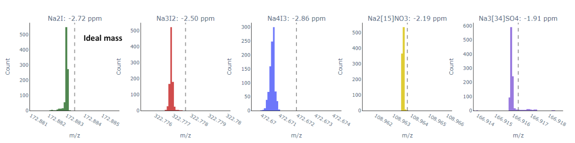
calibration_tolerance_ppm = 20# Set calibration tolerance to 20 ppm overlapped_scan_option = 1# Handle overlapping regions in neighboring segment scans (1 to enable handling)
# ========== 6. Parameters for Filtering and Clustering ========== # Pre-filtering based on "Air-beam" (Na2I range) Na2I_lower_bound, Na2I_upper_bound = 0, 50 * 1E6# Filter to remove bad air-beam ions
# Data size threshold for KDE clustering chunk data_size_threshold = 500# Minimum data size for performing KDE clustering
# KDE Parameters (for clustering noisy ions) kde_bandwidth = 0.0005# KDE bandwidth for peak density estimation kde_percentile = 5# Remove ions below the 5th percentile of density score (to filter out rare/noisy ions)
# DBSCAN Clustering Parameters eps_value = 0.5# Epsilon value for DBSCAN (maximum clustering distance in ppm) clustering_thre = 0.025# Retain clusters appearing more than 2.5% of Na2I showing frequency
# ========== 7. EESI-TOF reference ========== # tof_spectrum = pd.read_excel("./../Input/EESI-TOF_reference/EESI_LTOF_raw_curve_Punjab.xlsx") # tof_add_ion_threshold = 50 # 50 ppm means there is no Orbitrap ions within 50 ppm window of a EESI-TOF identifed peak apex # inorganic_ion_file = './../Input/EESI-TOF_reference/EESI_TOF_common_inorganic_ions.csv' # tof_peak_list_template = './../Input/EESI-TOF_reference/ToFware_peak_list_template.txt'
# ========== 8. Peak List Output and refining parameters ========== peak_list_prefix = './output/ToF_peak_list/20250720_Angola_Orbitrap+TOF_peak_list' refining_distance,refining_ratio = 25, 4
4. Applying the Reading data within user-defined time period
The segments refer to raw data extracted from the Orbitrap .ms1 text files, based on user-defined start and end retention times. Users can specify the desired time window for processing and optionally read multiple time segments to be merged in later steps.
1
2
3
4
5
6
7
8
9
10
11
12
13
14
15
16
17
18
retention_time_indices,rt_values = get_retention_time_indices(file_path, start_retention_time, end_retention_time) segments = read_ms1_segments_between_retention_times(file_path, retention_time_indices) df_segments = save_segments_as_dataframes(segments, pre_filtering_threshold) merged_spectrum = merge_segments(df_segments) merged_spectrum = merged_spectrum.sort_values(by = 'm/z', ascending=True) merged_spectrum = merged_spectrum.reset_index(drop=True) ``` The `showing_freq`, representing the recurrence frequency of a primary ion within the defined time window, is crucial for subsequent analysis. It reflects how consistently an ion appears and can serve as a basis for filtering other less stable or noise-like signals.
```python tolerance_ppm = 20## need to re-adjust based on the actual data peak_results = {} masses = [172.88347, 322.77771, 472.67196,622.566700,108.9638,166.9163]# for mass in masses: peaks = find_peak_near_mass(merged_spectrum, mass, tolerance_ppm) peak_results[mass] = peaks showing_freq = len(peak_results[masses[0]]) print (showing_freq)
We can also evaluate how closely the measured m/z values of calibrants match their theoretical values before applying calibration. This step is useful for pre-defining the tolerance_ppm parameter.
Comments